So you want to harness the power of machine learning but need a place to start? We've got just the task for you: detecting heart disease! Heart disease is the number one cause of death worldwide, so if you're looking to use data science for good you've come to the right place. To learn how to prevent heart disease we must first learn to reliably detect it. That's where you––yes you––come in!
 To join the competition, follow this link.
In our brand new warm up competition we're asking you to predict the presence or absence of heart disease given various data about a patient, including resting blood pressure, maximum heart rate, and EKG readings, as well as other information like age and sex. The data comes from the Statlog Heart dataset via the UCI Machine Learning repository. This is one of the smallest, least complex datasets on DrivenData, and a great place to dive into the world of data science competitions.
In this post, we'll walk through a very simple first pass model for predicting heart disease from patient data, showing you how to load the data, make some predictions, and then submit those predictions to the competition.
To get started, we import libraries for loading, manipulating, and visualizing the data.
%matplotlib inline

from pathlib import Path

import numpy as np
import pandas as pd

import matplotlib.pyplot as plt
import seaborn as sns
DATA_DIR = Path("..", "data", "final", "public")
Loading the Data
 Image and quote from the [Centers for Disease Control and Prevention](https://www.cdc.gov/heartdisease/facts.htm): As plaque builds up in the arteries of a person with heart disease, the inside of the arteries begins to narrow, which lessens or blocks the flow of blood. Plaques can also rupture (break open) and when they do a blood clot can form on the plaque, blocking the flow of blood.
On the data download page, we provide everything you need to get started:
- Training Values: These are the features you'll use to train a model. There are 13 features in data, including resting blood pressure, maximum heart rate, and EKG readings, as well as other information like age and sex. Each patient is identified by a unique (random)
patient_id, which you can use as an index. - Training Labels: These are the labels. Every
patient_idin the training values data has a corresponding label in this file. A0indicates no heart disease present, whereas a1indicates the presence of heart disease. - Test Values: These are the features you'll use to make predictions after training a model. We don't give you the labels for these samples, it's up to you to generate probabilities of the presence or ansence of heart disease for these
patient_ids! - Submission Format: This gives us the filenames and columns of our submission prediction, filled with all
0.5as a baseline. Your submission to the leaderboard must be in this exact form (with different prediction values, of course) in order to be scored successfully!
Since this is a benchmark, we're only going to use a subset of the features in the dataset. It's up to you to take advantage of all the information!
# for training our model
train_values = pd.read_csv(DATA_DIR / "train_values.csv", index_col="patient_id")
train_labels = pd.read_csv(DATA_DIR / "train_labels.csv", index_col="patient_id")
Let's take a look at the head of our training features
train_values.head()
train_values.dtypes
And the labels
train_labels.head()
Explore the Data
train_labels.heart_disease_present.value_counts().plot.bar(
    title="Number with Heart Disease"
)

The data is relatively well-balanced, so we won't take any steps here to equalize the classes.
selected_features = ["age", "sex", "max_heart_rate_achieved", "resting_blood_pressure"]
train_values_subset = train_values[selected_features]
A quick look at the relationships between our features and labels
sns.pairplot(
    train_values.join(train_labels), hue="heart_disease_present", vars=selected_features
)

The Error Metric – LogLoss
The metric in this competition is logarithmic loss, or log loss, which uses the probabilities of class predictions and the true class labels to generate a number that is closer to zero for better models, and exactly zero for a perfect model.
You can see from the formula for log loss that highly confident (probability close to one) wrong answers will contribute more to the total log loss number. This property of log loss makes it more informative alternative to accuracy. Below we'll use the Scikit Learn implementation of log loss to evaluate our model before submitting to the leaderboard.
Build the Model
When it comes to classic first pass models, few can contend with logisitc regression. This linear model is fast to train, easy to understand, and typically does pretty well "out of the box".
Below we'll combine the Scikit Learn logistic regression model with a preprocessing tool using Pipeline and GridSearchCV––two of sklearn's tools for streamlining the process of model training and hyperparamter optimization. You may be new to machine learning, but there's no better time to start developing good habits, and using pipelines is a good habit that you won't regret learning.
Logisitc Regression
# for preprocessing the data
from sklearn.preprocessing import StandardScaler

# the model
from sklearn.linear_model import LogisticRegression

# for combining the preprocess with model training
from sklearn.pipeline import Pipeline

# for optimizing parameters of the pipeline
from sklearn.model_selection import GridSearchCV
In Pipelines you pass a list of "steps" in the form of tuples with a step name in the first field and the object associated to the step in the second. Pipeline then creates one "estimator" object that you can pass data into for training and predcition.
pipe = Pipeline(steps=[("scale", StandardScaler()), ("logistic", LogisticRegression())])
pipe
Grid search allows you try out different parameters in the pipeline. Below, we try out different values for Scikit Learn's logistic regression "C" parameter as well as its regularization method.
To specify that these parameters are for the LogisticRegression part of the pipeline and not the StandardScaler part, the keys in our parameter grid (a python dictionary) take the form stepname__parametername. (Note the double underscore!)
The CV in GridSearchCV is another best practice to prevent overfitting your model.
param_grid = {
    "logistic__C": [0.0001, 0.001, 0.01, 1, 10],
    "logistic__penalty": ["l1", "l2"],
}
gs = GridSearchCV(estimator=pipe, param_grid=param_grid, cv=3)
With the parameter grid we've created and cross-validation, we're about to test 30 different models and take the best one!
gs.fit(train_values_subset, train_labels.heart_disease_present)
Let's take a look at the best parameters.
gs.best_params_
And the in-sample log loss score. Notice that since log loss wants the class probilities we call predict_proba and not simply predict, which would return the predicted labels, not their probabilites.
from sklearn.metrics import log_loss

in_sample_preds = gs.predict_proba(train_values[selected_features])
log_loss(train_labels.heart_disease_present, in_sample_preds)
Time to Predict and Submit
For the log loss, we'll be using the class probabilities, not the class predictions. This means we call the predict_proba method as above. Further, we'll take every row in the second column, which corresponds to the positive case of heart_disease_present.
Let's load up the data, process it, and see what we get on the leaderboard.
test_values = pd.read_csv(DATA_DIR / "test_values.csv", index_col="patient_id")
Select the subset of features we used to train the model.
test_values_subset = test_values[selected_features]
Make Predictions
Again, note that we take only the second column.
predictions = gs.predict_proba(test_values_subset)[:, 1]
Save Submission
We can use the column name and index from the submission format to ensure our predictions are in the form.
submission_format = pd.read_csv(
    DATA_DIR / "submission_format.csv", index_col="patient_id"
)
my_submission = pd.DataFrame(
    data=predictions, columns=submission_format.columns, index=submission_format.index
)
my_submission.head()
my_submission.to_csv("submission.csv")
Check the head of the saved file
!head submission.csv
Submit to leaderboard

Woohoo! It's a start! And that's exactly what we intend with these benchmarks. We're sure you'll be able to top this model in no time, and we can't wait to see what you come up with. Happy importing!